Saturday, 23 October 2021

Road Bike vs Gravel vs MTB speed test

Road bike versus gravel bike versus mountain bike (MTB) speed comparison
How much slower is a gravel bike than a road bike, on the road? 

How much slower is a mountain bike than a gravel bike? 

These are the questions I tried to answer with a quick test I did yesterday afternoon.  The results were a little surprising... 


The Bikes

Road Bike

A road bike from Planet X.

It has 50mm deep carbon wheels. The tyres are fast road bike tyres: Continental GP5000s with latex inner tubes.

Tyres were inflated to 80 psi.

It weighs around 7kg.


Gravel Bike

A titanium cyclocross bike from Planet X.

It's fitted with fairly fast small-knobbed gravel tyres (hence I'm calling it the "gravel bike"). The tyres are 43mm Panaracer GravelKing SK TLCs, run tubeless.

Tyres were inflated to 25 psi.

It weighs around 9kg.


Mountain Bike

A Scott hardtail.

On the front, it's fitted with a 2.25" Schwalbe Rocket Ron Snakeskin Addix Speed tyre. On the back, it has a 2.2" Continental Race King Protection tyre. Both are tubeless. These are both fast XC tyres.

Tyres were inflated to 22 psi.

It weighs around 9kg.


Clothing / Kit

For all three bikes, I wore the same road bike style kit, a tight fitting jersey and lycra shorts, base layer, standard helmet.  The same two bottles were used on all of the bikes.


Test Method

I rode the same 8 mile road circuit on all three bike, back-to-back during a 2 hour window.  It was fairly flat, with only 80m of climbing over those 8 miles.  I started with the road bike, then the gravel bike, then the MTB.

I recorded the speed on 7.5 mile stretch that was fairly uninterrupted. There was one set of traffic lights, at mile 5, where I had to stop the Garmin and re-start it. My average speeds that I extracted from Strava are not affected by the length of the stoppage at the lights.  Speed and position data was from GPS.

I tried to ensure a consistent effort on all three bike.  The road and gravel bikes both have Stages power meters. My previously power meter cross-calibration work showed that my road bike power meter over-reads by about 10W relative to my gravel bike's power meter. Hence I targeted 250W for the road bike and 240W as the target for the gravel bike.

My mountain bike doesn't have a power meter, so I had to go off feel, targeting the same rate of perceived exertion as for the other two.  I did however, have a heart rate monitor, and although I wasn't monitoring my HR during the test, my HR was close between all three bikes (Road Bike:160bpm, Gravel:157bpm, MTB:156bpm).  As a result, I was fairly satisfied that my effort and power was similar on all three bikes.

The geometry and position on the bikes is obviously different.  I chose to ride all three bikes in the style and position I would normally chose for riding each of those bikes.  Therefore, for the road bike, I was most stretched out and had the lowest torso.  I was most upright for the MTB. For the gravel bike, I was in between the other two. 


Results

As mentioned in the intro, the results were a little surprising:

   Road Bike:   20.2 mph / 32.5 kph,  245W average

   Gravel Bike: 18.5 mph / 29.8 kph, 239W average (=249W with +10W correction)

   MTB:            18.6 mph / 29.9 kph


So the Gravel bike was 8.5% slower than the road bike, which is close to what I expected.  The real surprise, though, is how fast the MTB was relative to the other two, and that it was marginally faster than the gravel bike!


Analysis

I created a segment in Strava, and used the Strava comparison feature to see how all three compared:

Gravel = Black (the reference), Road Bike = pinky purple, MTB = blue 
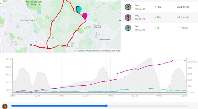
Road vs gravel CX vs MTB speed


Looking at this plot, it's clear that the road bike gains time on the other two everywhere.  Ignore the steps at ~4.3 miles, which is the traffic lights.  Stopping at the traffic light affects the segment times, which is based on clock time, but it doesn't affect the average speed, because I stopped my Garmin and is therefore based on time moving.

Then, the plot shows the MTB seems to gain time slightly on the uphill sections and lose time on the downhill sections.  The time losses on the faster downhill sections make sense, because the MTB and my position on the MTB is obviously less aerodynamic than the other two bikes.

It was strange, though, that it gained time on the gravel bike on the slower uphill sections. The two are similar in their weight.  Could it be the rolling resistance? Both gravel and MTB tyres were reasonably fast tyres, but the gravel bike tyres look like they should be faster.

To check this, I looked at the rolling resistance data on the Bicycle Rolling Resistance website, which is an excellent resource that I use to help me choose tyres.  I was familiar with rolling resistance data for all my sets of tyres, versus alternative choices in their categories, but I'd never compared the rolling resistance of gravel and MTB tyres against each other. To my surprise, the MTB tyres are actually lower rolling resistance that the gravel tyres:

Gravel Tyres: 56.6W @27psi,  49.4W @36psi -> 65.4W at the 25psi pressure ridden

                         -8W adjustment for tubeless setup -> 57.4W at the 25psi pressure ridden

MTB Front tyre: 48.6W @35psi, 53.4W @25psi -> 59.6W at the 22psi pressure ridden

MTB Rear tyre: 36.0W @35psi, 40.4W @25psi -> 46.1W at the 22psi pressure ridden

MTB average: 52.8W assuming 50/50 front/rear weight split (for simplicity)

                         -10W adjustment for tubeless setup -> 42.8W at the 22psi pressure ridden

All power values above are for two tyres at 85kg load at 18mph, which is quite close to my test conditions.  The GravelKing tyre data was for 38mm version, but recent testing on the BicycleRollingResistance website has shown that the performance difference between 35mm and 40mm versions of the GravelKing TLC is very similar, so using the data from the 38mm version is good enough I think.  Both rolling resistance numbers have been adjusted based for tubeless a tubeless set-up, because the standard testing uses butyl inner tubes. The MTB tyre power number was reduced by 10W, based on this BicycleRollingResistance data.  The gravel tyre power number was reduced by an estimated 8W, estimated by looking at how latex tube versus butyl tubes affected the MTB and road bike power numbers.

Something to note is that I am running foam tyre inserts in my Gravel tyres, although I took care to ensure the tyre inserts are not contacting the tyre and getting compressed at the contact patch (and with some margin to spare), to ensure the tyre inserts don't affect rolling resistance.

For reference, the road bike tyres are much lower rolling resistance than both the gravel and MTB tyres:

Road Bike tyres: 20.0W for a GP5000 with latex tubes at 80 psi, i.e. a 23-37 Watt advantage over both the MTB and gravel bike tyres.


Discussion & Conclusion

The results surprised me, but upon closer inspection it's clear that the MTB has an (unexpected) 14.6 Watt rolling resistance advantage of the gravel bike.  This seems to have an beneficial effect at the slower speeds, when the aerodynamic disadvantages of the MTB are less dominant, and overall it gave the MTB a marginally higher speed one the 7.5 mile road route.

We have to keep in mind that the MTB did not have a power meter, but nevertheless I took care not to go 'too hard' on the MTB, by riding that bike last (when I was most fatigued), and by checking my heart rate data after the ride, to ensure it was not higher than for the other two bikes. 

This leads me to now wonder: If my gravel bike isn't faster than the MTB on a flat-ish road route, in what situation would the gravel bike be better than the MTB, if any?? 


Saturday, 18 September 2021

Stiff pedal bearings/seals - What's the power loss?


Power loss from stiff pedals

The other day, one of my friends commented in our bike chat WhatsApp group about his flat pedals and how they were "quite stiff".  He was wondering how much power this would be costing him.

I told him that if he was curious enough to spend a few minutes looking into it, he could measure the resistive torque and calculate the associated power loss from that.

I did a back-of-the-envelope calculation of the power cost, based on 80 rpm cadence (see below).

The resistive torque he can feel when turns the pedals is either coming from either poor bearings, or more likely (as the pedals were new), from stiff seals.

I told him he could measure the resistive torque by hanging a weight off the pedal and measure the distance from the pedal axle.  Progressively adding weight until the pedal turned would then give a resistive torque (weight in Newtons multiplied by moment arm). Multiplying by cadence in rad/s then provided the power lost for one pedal.  Multiply by two to give total bike power loss.  Strictly speaking, what's measured with this method is stiction, or rather the resistive torque due to stiction, whereas we really want the friction losses when the pedal is turning. That's more difficult to measure simply though.  I think the stiction torque would give a conservative (slightly high) estimate of the power cost, which is good enough I think.

The results?  He found he needed 161g of weight at a 5cm moment arm to turn the pedal.  He calculated this to be 1.35 Watts of power loss using my equation below.  So not significant, but not nothing either.


Thursday, 19 August 2021

Time trial aero improvements


CdA time trial improvements
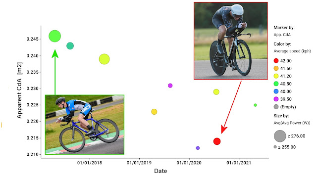
This plot shows my improvements in my 10 mile time trial performance over the last 4 years.

I have been doing time trials since about 2017, having converted my old winter road bike to a time trial bike, using a set of clip-on aero bars.

Over the last 4 years, I've made various improvements to the bike, my kit, and more importantly my position on the bike.

My time trial times have gradually improved.  Not significantly so, but considering my power hasn't really improved during that time, these speed improvements are a result of improvements to my equipment and position.

I do a combination of local club 10 mile evening time trials and also 10 mile TTs organised by DBmax at the local Castle Combe motor racing circuit.  I used the data collected from these Castle Combe time trials to analyse my improvements in performance, particularly my aerodynamic efficiency (CdA), which is a parameter that's critical for good time trial performance.

2017 Equipment

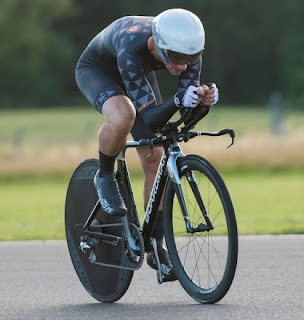
This photo shows my setup in 2017, which was my first Castle Combe 10 mile TT:

- Ribble Audax aluminium frameset.
- Superstar Components 46/66 carbon wheels
- 3T aluminium base bar
- 2nd hand clip-on hand aero bars
- Regular bib shorts and jersey
- Specialized Evade aero road helmet
- Velotoze shoe covers


Over the last few years, I made a number of improvements.  Often, when I had to make a choice about equipment or kit selection, to decide which was fastest, I did aero testing using the Chung Virtual Elevation Method to determine the CdA of various set-ups.  I haven't been exhaustive in my Chung testing, because it’s quite time consuming to do properly, for every change.  However, I've used it for a few things, for example to compare two different helmets and two different skinsuits.

The plot at the top of this post shows the improvements in my apparent CdA over time, determined using the free Golden Cheetah Aerolab software.  This type of CdA calculation assumes no wind, hence I call it 'apparent CdA'.  Furthermore, for all data points, I have assumed similar values for weight and rolling resistance.  Consequently, any improvements in either of those two things will appear as benefits in the apparent CdA value. My weight and the rolling resistance of my tyres has been reasonably consistent though, so this is an acceptable simplification I think.

The largest improvements in CdA seem to have come from lowering my aerobars, allowing me to get my back flatter and my head lower.  I haven't specifically tested bar height via Chung testing, but the biggest improvements in CdA seem to correlate with bar height.  Interestingly, the bar height adjustment was the cheapest upgrade of all, costing me just £15 for an adjustable stem from Decathlon.  All other kit upgrades, costing probably £1000-£1500, didn't seem to be as effective at reducing my CdA.  So the best modification was also the cheapest one.

Subjectively, my position now looks much better on the bike.  In addition to my position changes, I've also improved the bike and kit: 

2020/2021 Equipment

- Boardman Air TT carbon frameset.
- Wiggle Prime Black 50mm front wheel.
- Planet X disc rear wheel
- Single 50t front chainring
- Bell Javelin 2nd hand helmet
- Bioracer/Nopinz Speed Concept skinsuit


A few things were unchanged from my 2017 setup:
- 3T aluminium base bar
- 2nd hand clip-on hand aero bars
- Velotoze shoe covers


Speed Improvements

The plot below shows the improvements in my CdA over time, as a result of the bike and positions improvements I've made.  The colour of the points indicates the average speed for each 10 mile TT.  The size of the circular points indicates that average power I managed to achieve.


As can be sWhat's clear from the plot above is that the fastest times were not achieved with the highest power (largest circles), but actually the speed is a function of both power and CdA.  In fact, it's clear from the speeds that a reduction in power, often a result of being lower at the front, is more than compensated by an improvement in CdA, resulting in net benefit for the average speed.

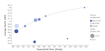
For time trials, it's often said that you want to maximise Power divided by CdA.  All things being equal, a time trial average speed will be dependent on this parameter, Power/CdA.  For example, if CdA can be reduced by 10%, then the power required to maintain the same speed also drops by 10%, simple as that.

I wanted to see how my time trial average speeds correlated with Power/CdA.  However, since I was comparing time trial performances on different days, I also wanted to account for changes in air density from day to day, since air density directly affects aerodynamic drag and therefore speed.  Lowering the air density by 10% has the same effect as reducing the CdA by 10%.  The air density effect can be incorporated by considering Power/[CdA*Rho] as the parameter to plot speed against, instead of Power/[CdA].


The plot below shows how my average time trial speeds correlate against Power/[CdA*Rho].


In the plot above that you can see that my average speed generally correlates well with Power/[CdA*Rho].  There are, however, two annoying outliers where my speed was very low considering my average power, the air density and my apparent CdA.  I don't yet understand what has caused these two outliers.  I've checked my Golden Cheetah virtual elevation calculation (the CdA calculation) and those seem fine.  It might be something as simple as a badly calibrated speed sensor or a power meter that hasn't been zero'd.


Sunday, 7 February 2021

Real life speeds versus virtual cycling speeds


Comparison of RGT Cycling virtual speeds versus real life cycling speeds
I like the RGT Cycling virtual cycling app.  Unlike Zwift, it has a neat feature that allows you to create 'magic roads', which are virtual roads created from real road GPX data.  Anybody can upload GPX data to create a magic road.

This allows you to ride real roads inside RGT Cycling, so either local roads that you've ridden already, or famous roads that you'd like to ride (created by other people).

In this time of COVID-19 restrictions, it means that virtual races can be organised on real racing circuits, which is pretty cool.  Somebody else has already uploaded my local Odd Down Cycle Racing Circuit to the magicroads.org website.  Virtual races are being organised by PDQ Cycle Coaching, the guys that organised the real life races I did back in 2019.


Odd Down Cycle Circuit
The Odd Down Cycle Circuit is located near Bath, in the South West of England.  It's a 1-mile circuit, with very mild elevation changes and a couple of hairpins that can be taken at speeds below about 20-25 mph.

RGT Cycling also prides itself on providing a realistic virtual cycling simulation, which is something I like.  They strive to get the modelling accurate and the app includes features like braking and speed limits around tight corners, which is something that's different to Zwift, for example.

I thought it would be interesting to compare my real life cycling speeds around the Odd Down Circuit with the virtual speeds achieved in RGT Cycling.


Real life speeds

PDQ Cycle Coaching Odd Down 4th Cat Race 2019
I extracted speeds from three races I did in Spring/Summer of 2019.  I only extracted speed from the warm up laps, not the races themselves, so that the speed would not be subject to drafting.  The average power during these warm ups varied from about 150W to 260W.  I usually do a ramp-type warm up, with the power held constant for 2-3 minutes at a time before increasing it. Therefore, most of the warm-up laps were done at roughly constant power.

The data from three separate warm ups (three different days) allowed some checking of the influence of external weather conditions, which would affect average speeds.  Lap speeds were obtained from Strava for the one-lap segment that has been created in Strava.  Results are shown below with blue symbols.

Comparison of RGT Cycling virtual speeds versus real life cycling speeds

I also wanted to check my CdA because any speed discrepancies with RGT could be due to different CdA assumptions by RGT.  I estimated my CdA by loading my warm up GPX data into Golden Cheetah and using the Aerolab Chung method virtual elevation plots to determine CdA.  My CdA could be estimated for two of the three warm ups, and was 0.360 and 0.375 m^2 for those two warm ups.  I had to make some assumptions/guesses about the rolling resistance coefficient (CRR=0.004), the drivetrain efficiency (97%), my total weight (80kg) and the air density (1.2 kg/m3).  It's worth noting that my warm up laps were done on the hoods, with fairly straight arms, whereas my RGT avatar drops into a more aerodynamic horizontal forearm position when speeds are above about 25 kph (15 mph), which is most of the lap. 


RGT Virtual Speeds

RGT Cycling Odd Down
I rode the Odd Down Circuit in RGT Cycling on Saturday 6th Feb 2021, selecting no bots, so that my riding would be solo, with no drafting.  The speeds were measured in the same way, using a Strava segment, and are shown with the red symbols on the plot above.  The RGT ride was also loaded into Golden Cheetah, making similar assumptions about CRR=0.004, drivetrain efficiency (97%), weight (80 kg) and air density (1.2 kg/m3).  This gave a CdA value of 0.285, which is quite a lot smaller that my real life CdA of 0.360-0.375.  Incidentally, I saw a tweet from Robert Chung a while ago, saying that he had found that Zwift also assumes a rather optimistic CdA of 0.28.


Differences and possible reasons

The general agreement in the plot above seems to be not too bad on the face of it, but it's not great either.  The RGT speeds are approximately 1-2 mph higher, and this I think comes primarily from the lower CdA assumed by RGT.  The difference of CdA, 0.285 in RGT versus 0.370 in real life, is quite significant.  That difference would result in a speed difference of 1mph at 250W, or about 30W at a fixed speed.

Of course, RGT is not trying to simulate me personally, and it has no idea how aerodynamic my bike and body combination is, or was during those warm ups.  It's worth bearing in mind that my warm up laps were done on the hoods with fairly straight arms, so that position will be less aerodynamic than what RGT is assuming.  I also wasn't wearing a skinsuit, and hadn't shaved my legs, both of which the RGT avatar has.  These are differences that Specialized have shown in their videos have a significant effect on aerodynamic efficiency.

It's also worth noting that I used the same power meter for all rides, including indoor RGT ride, so there should not be a bias coming from using different power meters.  It is possible that my left crank only power meter is slightly over-estimating my power, and there is some evidence of this based on recent testing.  An over-estimated power would result in RGT speeds that are higher than real life, and could also partially account for the different apparent CdA values. 

Overall though, I think the differences are primarily coming from the different riding position that RGT is assuming (horizontal forearms), relative to the position I adopted during my real life warm ups (almost straight arms, more upright torso).  Wind tunnel test performed by Aerocoach in 2019 showed that dropping the elbows into a horizontal forearm position ('breakaway hoods') significantly reduced Xavier Disley's CdA from 0.3506 m^2 to 0.2718 m^2.  This reduction of around 0.08 m^2 is very similar to the CdA differences extracted from my RGT ride and my real life rides, for similar changes in position.  Therefore, I conclude that the RGT cycling simulation is accurate, once you factor in the cycling positions that are assumed and adopted by the RGT avatar.

Besides this quantitative comparison of speeds, there is a qualitative element too, particularly around the cornering.  I found the RGT simulation of corners to be fairly realistic.  In real races, I usually have to brake for the hairpins due to the concertina effects when riding in the bunch.  During warm ups or solo breakaways, though, I often don't need to brake.  I remember holding about 280W during one solo breakaway and not needing to brake, although that was very close to the limit.  In RGT, the same thing happened, with just a momentary 1-2 seconds of braking before the bottom hairpin during the laps at 270W.  Qualitatively, this seemed to agree with real life, although it's difficult to be too conclusive.


Conclusion

All in all, I'd say that the RGT simulation is a realistic simulation of real life riding around my local Odd Down Cycle Circuit.  Where differences exist, I think there are some plausible explanations for what might be causing those discrepancies.  


Sunday, 31 January 2021

A quick attempt at real-time CdA measurement


Real time (instantaneous) CdA bike drag extraction
This post describes my attempt to calculate the real-time (instantaneous) drag that I'm experiencing when I'm on my time trial bike, using data from my power meter, altimeter and speed sensors.

For several years now, I've been measuring and trying to improve the aerodynamic drag of my time trial bike.  For time trials, the aerodynamic drag is critical to how fast you can go, because on a flat road most of your power (~80% of it) is expended to overcome the aerodynamic drag.  Put simply, if you can improve your aerodynamic efficiency (your "CdA") by let's say 10%, you can reduce the power needed by around 10% while maintaining the same speed.  Alternatively, you will go faster for the same power.


What is CdA?

Aerodynamic efficiency is defined for cyclist using a parameter called CdA.  In fact CdA is two parameters, multiplied together: Drag coefficient (Cd) and frontal area (A).  The drag coefficient defines how aerodynamically efficient a certain shape is, regardless of its physical size.  For example, a beach ball and a baseball will both have the same drag coefficient*, Cd, because they have the same shape (a sphere), even though they are obviously different in  size.  If both balls are subjected to the same air speed though, the larger beach ball will experience a larger drag force in Newtons, because it has a larger frontal area (A).  In fact, the drag force will be ten times greater, for example, if it's frontal area is ten times greater than the baseball.  Therefore, it's convenient when we are adjusting both the shape of a bike/rider (Cd), and also the frontal area (A), as we usually do when adjusting a time trial set-up, to combine both of these parameters.  It is the product of these two parameters (CdA) that we want to minimize in order to go faster.

* There are a few caveats to this statement, but I won't go into those details here.

The Virtual Elevation Method (aka The Chung Method)

In the last decade, the excellent virtual elevation method, invented by Robert Chung, has become the standard method for triathletes and time trialists to measure their CdA in the field (i.e. on standard roads, not in wind tunnels or velodromes).  Additional information about the method can be found on the Slowtwitch Platypus Thread.

I have been successfully using this method for several years to measure and improve my CdA.  The trouble with it is, though, it's quite time-consuming to collect and analyse the data.  The way I do testing, to test two bike setups, back-to-back, then to repeat them to be sure ('ABAB' testing), takes about 40 minutes of riding time, with about 10 minutes per setup. The analysis of the results probably then takes another 30 minutes to 1 hour, once I'm back home. 


Real-time CdA

I wanted to see how feasible it would be to extract the CdA value in 'real-time'.  That is, at 1 second intervals, could you extract the CdA based on the measured power, elevation and speed?  All of that data is used by the Chung method, but it is processed in a different way, to give you the 'average' CdA over the run.  To extract real-time CdA, you simply solve the power equation on slide 14 of Robert Chung’s VE presentation to solve CdA, using the instantaneous measured elevation, instead of the usual procedure of guessing a value for CdA and then solving elevation.

I attempted to extract real-time CdA using data from a 10-mile time trial I did in 2019.  I didn’t have high hopes that it would be successful, but I was curious anyway and wanted to give it a go.

My findings? Well, the noise in the resulting real-time CdA values was even worse than I expected, with real time CdA values ranging from -1.4 to +1.0 m^2!  (the green trace in the Figure 2).  The average of the real time CdA data, over the 10 miles, was actually relatively good, agreeing with the CdA from my virtual elevation analysis to within 0.01m^2 (0.220 vs 0.213, as shown in Figure 1).  However, the noise in the real-time drag clearly makes it unusable as a drag extraction method though.


Castle Combe Chung Method virtual elevation CdA analysis
Figure 1: Virtual elevation (Chung method) CdA calculation


Real time (instantaneous) CdA bike drag extraction

Figure 2: Real Time (instantaneous) CdA calculation


What I realised is that the noise in the CdA calculations, to a large extent, comes from the poor precision of my Garmin’s elevation measurements, coupled with sensitivity of the CdA calculation to elevation errors.
 My Garmin elevation data has a precision of 0.4m (or at least I see 0.4m increments in its output).

The high sensitivity of the real time drag to elevation is best explained with an example, assuming the following:

Mass = 80 kg rider+bike, Speed = 45 kph, CdA = 0.217 m^2, CRR = 0.004, Power = 300W, Rho = 1.2 kg/m^3, 97% transmission efficiency.

In this example, 252W is overcoming aerodynamic drag.  A 10cm increase (or error) in elevation over a 1 second period equates to a slope of 0.8%, is 78 Joules of potential energy (80*9.81*0.1) and is therefore 78 Watts that gets injected into the power balance equation.  This results in a 31% reduction in the real time CdA ((252-78)/252) if speed remains fixed.  Of course, if the elevation really did increase by 10cm, there would be an associated reduction in speed for a constant power, which would offset the potential energy change, and the CdA would remain the same.  However, the precision of the Garmin barometer means that large elevation steps (40 cm in my data) were introduced into the real-time CdA calculation, causing the CdA spikes.

This sensitivity to elevation data can be mitigated by using longer sampling periods, for example 30 seconds, as shown in the dark green curve in Figure 2.  Alternatively, or in addition, more accurate elevation data would help, and I know there are some folks (for example, see here) that are using more precise barometric sensors to help with this.  The example above, though, shows it’s a tough problem to crack.  Even a really small 1cm elevation error would be a 3% drag change over 1 second.

The beauty of the Chung Method, the way I see it, is that it disregards this instantaneous elevation data that CdA is so sensitive too, and instead calibrates to known elevation information over a longer time period, thereby elegantly avoiding this difficulty.  Another alternative to avoid this elevation sensitivity, of course, would be to ride a perfectly flat road like a velodrome.  However, I’m lazy and would prefer to do my testing 5 minutes away from my home!


Conclusion 

This exercise, although it was generally unsuccessful, was useful in showing why the Chung Method works so well, by avoiding the use of inaccurate elevation data that would otherwise cause difficulties.

It also shows that it's incredibly difficult to extract your instantaneous CdA value, using the power data from your power meter.  On a perfectly flat road it would be feasible, but not on a random road where you have to rely on measured elevation.  The idea of looking down at your head unit, and to see your CdA displayed (as you do for your power or speed), would be brilliant.  Unfortunately it seems that would be very difficult to achieve.


Thursday, 14 January 2021

1x (single chainring) conversion for Shimano 105 chainset


1x single ring Gravel/Cyclocross conversion for Shimano 105 chainset
This is my Shimano 105 chainset that I've converted to a 1x system.

Buying a brand new 105 chainset and then converting it to a 1x single chainring setup was, surprisingly, both cheaper and also lighter than buying a dedicated Shimano GRX 810-1 1x chainset.

Previously, I had a SRAM Rival chainset on my cyclocross/gravel bike.  I wanted to swap my Rival chainset for a Shimano one, so that I could then install a Stages Shimano power meter, which would be the same brand and type of power meter as what's on my road bikes.

If I had bought a Stages GXP power meter that would have been more expensive than the 105 power meter and also would not have been interchangeable with my other bikes.  Initially I planned to get Shimano GRX 1x chainset and a GRX or 105 power meter. However, I learnt that Shimano has created the GRX groupset to have a slightly wider Q-factor than the Q-factors of their road groupsets, like 105 etc.  This, again, would have meant the GRX power meter would not have been interchangeable with my other bikes, should I ever want to swap them around in the future (albeit with a Q-factor difference that is very small).

I decided instead that I'd get a new 105 chainset, convert it to a 1x single chainring set-up, and couple that with 105 Stages power meter.  Surprisingly, this 105 1x setup is both lighter and cheaper than the top level GRX 1x 810-1.  Comparisons are made against the more expensive and lighter 810 version of GRX.  Shimano also make a cheaper, heavier GRX 600 groupset too.

A comparison of prices and weights is shown below:

  Shimano GRX 810-1 42t      Shimano 105 1x 42t     Difference
RRP   £214.99         £186.59     £28.40
Current Wiggle Price   £179.99      £168.19     £11.80
Weight   656g      632g      24g

Cost and weight breakdown:
Shimano 105 5800 chainset without rings & bolts:  £154.99 RRP,  £136.39 current Wiggle price, 549g  
4 x chainring bolts:  £5.19 from Ebay, 6g
42t J&L wide/narrow chainring: 26.60 from Ebay, 77g
All 105 and 1x components were weighed myself.  GRX weights were taken from Shimano website

Sunday, 27 December 2020

Low cost, space saving squat rack


Low cost, space saving, DIY home squat rack

With gyms closed for most of 2020, due to COVID-19, I decided to set-up my old weight bench and start doing my strength training at home instead.  What I've always lacked, though, is a squat rack.

The problem is, squat racks are expensive.  At least £130 for a cheap, non-adjustable one.  I can't justify that expense, considering the modest amount of strength training I actually do each week.  Also, they take up a lot of space, having a large footprint. It's space that I don't have in my garage.  

My solution has been to build a rack that hangs from the garage ceiling rafters to support the barbell. The function of the lower 'bar catchers'/spotters on a proper squat rack is then achieved using Olympic gymnastic rings and straps.

The timber, hooks and coach bolts cost about £25 from B&Q and Screwfix.  The hooks were rated as 90kg load capacity each (180kg total for two). I'm currently squatting about 70-80kg, so that will be plenty strong enough.  The gymnastic rings and straps cost £10 from Ebay. When I'm not using it, the timbers arms fold upwards and hook onto the ceiling, out of the way.  The video below best shows how it works.


Monday, 7 December 2020

Stages Power Meter Cross-Calibration


Cross-calibration of Stages Power MeterI recently bought a new Stages 3rd generation power meter (PM) for my new gravel bike.

This is the third power meter I now own, with the other two also being Stages PMs. The other two PMs I own are on my road bike and my time trial bike (a 1st gen and 2nd gen Stages PM respectively).

I decided to buy another Stages, partly because Stages PMs are good value for money (this third one was less than £300 brand new), and partly because I was keen to have the same brand of PM on all bikes.  My hope was that by having the same brand of PM, they would deliver consistent power values between the three devices.  However, I wanted to check how consistent they actually are...


Method

The best way to do this, I decided was to use my Wahoo Kickr Smart trainer as the 'balance'.  In general, the power numbers from smart trainers are not considered to be as accurate as those from dedicated power meters. However, with some care, the power values from the my Kickr smart trainer should at least be consistent, meaning that my Kickr could be used a common power source to enable the other devices to be compared with each other.  The agreement with the values from the Kickr is unimportant.

Some care was taken to ensure consistent testing of the three devices
  • Testing was done in the same gear, 50t front, 16t cassette, and at the same cadence (85rpm)
  • The same pedals and RH crank/chainrings were use for each PM test.
  • All PMs were stored in the same place (same temperature) before installation.
  • The Kickr smart trainer was connected via bluetooth to my iphone.  The power meter was connected with ANT+ to my Garmin Edge 520, to provide independent recording methods.
  • Exactly the same PM installation sequence was done each time.
  • The same testing protocol was done for each PM.
The protocol for the testing was as follows:
  1. With no power meter installed, I warmed up the smart trainer for 15 minutes at 140-170 Watts.
  2. The smart trainer was then calibrated. No further re-calibration of the trainer was done.
Then, for each of the three power meters, the following was done:
  1. Install the first power meter. LH crank bolts tightened to 12Nm.
  2. Power meter calibrated (zero offset) via the Stages app.
  3. Collected power data at the first power setting, 150W:
    • Use TrainerRoad app to set the smart trainer target power to 150W in ERG mode.
    • Pedal for 1 minute to allow everything to stabilise.
    • Press the lap button, and pedal for a further 2 minutes to collect power data.
    • Record the average power from the power meter (Garmin) over the two minutes.
  4. Collect power data at second power setting, 215W, using the same steps.
  5. Collect power data at third power setting, 280W, using the same steps.
  6. Optional: Collect repeat power data at 215W and 150W if time, energy, and motivation permit.
The order of testing the power meters was:
  1) Stages Shimano 105 7000 Gen 3 power meter
  2) Stages Shimano 105 5800 Gen 2 power meter
  3) Stages Shimano Ultegra 6700 Gen 1 power meter

4) A fourth run was done with a repeat of (1), the 105 7000 Gen 3 power meter, to check the repeatability after a PM re-installation.


Results

Cross calibration of Stages power meter using Wahoo Kickr

Repeatability

You can see from the plot above, that there's a fair amount of variation seen in the results, not just between the three power meters but also some significant changes seen in the repeats.  Ideally, the repeats should be very close to the first recordings, so what can we learn from this?

Starting with the repeats, the installation repeat run gave some differences of 2-11 Watts between run (1) and run (4) for the same power meter. There are several possible explanations for this difference that I can think of:

Explanation 1) The Stages power meter calibration drifted between runs 1 and 4.  This is unlikely because both runs were done with exactly the same protocol, so there is no additional usage of the PM that should cause a drift. For example, it was no warmer on the 4th run, having been inactive for 45-60 minutes.  Also, the differences between the powers are not consistent across the range, so it's not a parallel offset that would otherwise indicate a calibration drift.

Explanation 2)  The Wahoo Smart trainer has drifted.  Again, I think this is unlikely because if this were true, I'd again expect a constant parallel offset to be seen between runs 1 and 4.

Explanation 3) The most likely hypothesis is, I think, that both runs are subject to small changes in my left/right leg balance, with random changes affecting the results.  For example, if at 150W I have a 48/52% left/right leg split, then the left leg produces 72W, the right leg produces 78W to create the 150W (real) power total. However, the Stages PM always assumes the right leg also produces the same as the left, 72W, so the Stages PM would give a total power of 144W. If that L/R balance then swings by 4% to 52/48% L/R instead, then the left leg produces 78W, the right leg produces 72W, but the Stages PM gives a total power of 156W.  So a swing of 2% asymmetry to the left, to 2% assymmetry to the right, will create an apparent power difference of 12W for the same actual 150W power total in both cases.  If the target power is higher, say 280W, that same swing would be higher, 22.4W.

I think this is third explanation, of random small changes to the L/R leg imbalance, is the most plausible explanation of the 2-11 Watt variation seen in the installation repeat. It also explains why similarly large differences are seen in the repeats that were done before uninstalling each power meter (step 6 in the method).

Power meter differences

The differences between the power meter results has to be considered with a view of these repeatability results.  However, even considering the repeatability, and the uncertainty that it introduces, I feel the Gen 2 105 power meter (the red data points) is reading higher that the other two PMs.  Although its difficult to be conclusive, I would say the the Gen 2 105 PM is reading around 10-Watts higher than the other two.

This isn't a huge difference, but it is large enough that I'll need to take it into consideration when riding close to my limit, close to threshold.  This Gen 3 105 PM will go onto my gravel bike, with the Gen 2 staying on my Road bike, which I use for most training, FTP tests etc.  I will therefore have to keep in mind that the power values on my gravel bike may read a little low compared with what I am used to on my road bike, for the same effort level. 

Friday, 13 November 2020

Upgrade recommendations for a friend

In a 2016 blog post, I described an analysis that concluded about the best value for money upgrades that people can buy for their road bikes.

Last week, in my previous post, I described the power delivery optimisation that I did for my friend Steve, to show how much faster he could go just by changing when he pushed harder on his favourite bike route and when to ease off.  I followed this up with a quick study to show how much benefit could be achieved with certain bike and kit upgrades.

The analysis I did was basically the same as the 2016 analysis, except it was done for Steve's lunchtime bike route, instead or three generic bike ride profiles.  The results are shown in the bubble plot above.  I've shown it with upgrade price on the x-axis, and the equivalent power saving in the y-axis.  Items that represent the best value for money (Watt saving per £ spent) have the largest bubbles.

The conclusions are similar to those in the 2016 blog post.  Buying latex tubes represents excellent value for money, probably the best there is.  On the other hand, paying extra money for a lighter groupset (if it has no additional functional benefits) is a really bad way to spend your money, if improved cycling performance is your priority.


Wednesday, 11 November 2020

Power delivery optimisation for a real-life cycling route


How to improve you average speed cycling
In a previous blog post (here) I described a power delivery optimisation analysis that I did back in 2016.  In that work I showed that, using a simple Excel-based optimiser, it's possible to make significant performance gains, a 2-3% improvement in that case, simply by optimising the power delivered during a bike ride for the same normalised power.  In other words, making the most of what you've got.  These improvements were the versus the 'baseline' situation where the ride was done at a fixed (not varying) power output with the same normalised power.  A 2-3% improvement may not sound like much, but to put this into context, that performance gain is equivalent to a 5% power improvement, for a fixed power delivery.  Alternatively, it's equivalent to a 5-6kg of weight loss, which is significant.

That study was done for a fictional 80km route having 1000m of elevation gain.  In 2020, a friend of mine, Steve, who's also an engineer, asked me if there was a better way for him to ride his favourite lunchtime cycle loop.  To give him some advice, I decided to try putting his bike route into my Excel optimiser to see what it would give.  By optimising his power, using the optimised power profile shown in the plot above, he could make an impressive 3.8% time saving and speed improvement, compared with riding the route at a fixed (constant) power.  This blog post describes that work in more detail.


Route setup

First I extracted my friend Steve's lunchtime route from Strava, as a GPX file.  That Strava output gave 276 waypoints on the route, with longitude, latitude and elevation data.

For my optimiser to work, I needed to reduce the number of points to 137 points, which is a number of segments that would be compatible with what Excel's optimiser can handle.

Steve's best time for this ride was 29 minutes, 42 seconds, which was an average speed of 31.8 kph.  I obtained a few other parameters from the  Strava file for his personal best time, then I needed to guess a few others:

Ambient temperature = 6 deg C  (from Strava)
Ambient Pressure = 101.25 Pa  (assumed)
Bike + Rider = 97.5 kg  (estimated)
Mechanical efficiency = 97.5%  (assumed)
No wind  (assumed)

Comparison with BestBikeSplit

As a first check that my optimiser was doing something sensible, I compared the output with
BestBikeSplit.  BestBikeSplit does something very similar, so both methods should give reasonably similar results.  

BestBikeSplit assumed a rolling resistance coefficent (CRR) of 0.00622 and a CdA of 0.3424 [an explanation of CdA can be found here].  I
 used those two values in my own optimiser.  As can be seen from the plot on the left, both methods gave reasonably similar results for a normalised power of 239W:

BestBikeSplit: 29.8 kph average speed
My optimiser: 30.7 kph average speed

Qualitatively, the power distributions in those plots look similar.  The BestBikeSplit optimiser can split the route into only 50 segments, whereas my optimiser used 137 segments. This might be a reason why the average speeds differ slightly.  In any case, I was satisfied that this agreement was close enough.

Tuning CdA

I then tuned the value of CdA so that the optimised ride time was equal to Steve's best ride time.  Reducing CdA to 0.29 was enough to do this, to increase the average speed from 30.7 kph (for a CdA of 0.3424) to 31.8 kph for a CdA of 0.29.  A CdA value of 0.29 is a bit low for a recreational cyclist, in my experience, but Steve often rides with one of two colleagues, so 0.29 seems a reasonable value for his effective CdA, considering that some of the time he'd be riding in the draft of other people.

For this CdA of 0.29, and for a normalised power of 259.8W, I computed the "weighted average power" to be 241.0W and the average power to be 227.3W.

At this point I should note that the way in which Strava calculates weighted average power is not documented anywhere by Strava.  Weighted average values are generally higher than the average power values in my experience, but are always less than normalised power values.  Whereas normalised power is calculated by raising the power values to the power of 4, I assumed that weighted power is calculated by raising the power values to the power of 2.

So to summarise, I now had an optimised power profile (see plot on the left) that produced an average speed that is identical to Steve's PB effort (31.8kph) using the same weighted average power as he produced in real life (241W).  Of course, it's highly unlikely that he would have ridden the route at the optimum power profile, but for the purposes of this study, to quantify the benefits of optimising power, I think that's good enough.  As an observation, it's interesting to see that the power needed to produce this optimised performance varies significantly, from about 20W on the steepest downhill part of the route (-10% gradient) to about 370W on the steepest uphill part of the route (+8% gradient).  Incidentally, the average power and normalised power for this power delivery is 227W and 260W respectively.

The improvement that the optimised power delivery achieves, versus the baseline case of a fixed, non-varying, power delivery can then be calculated by re-running my optimiser with an additional constraint.

How much faster is the optimised power delivery?

I re-ran the optimiser with weighted average power set to 241W, as before, but this time I also set an additional constraint that the average power had to be 241W too.  This additional average power constraint effectively prevented any significant variation in the power, meaning that the power delivery effectively became almost constant at 241W, as shown in the plot above.

The speed of this ride, if performed at this fixed power of 241W, would be 30.6 kph.  This is 1.2 kph slower (3.8% slower) than for the ride done at the optimised power delivery.

Comparison to other improvements

The significance of this 3.8% improvement is not so obvious, but can be put into context by calculating the effect of other improvements:

+10 Watts increase in weighted average power:            +0.7kph improvement (2.2% faster)
Butyl -> Latex inner tubes (-11% rolling resistance):      +0.3kph improvement (1.1% faster)
5 kg weight saving:                                                         +0.5kph improvement (1.5% faster)
Aero improvement through and aero helmet upgrade:   +0.2kph improvement (0.8% faster)

The speed improvements shown above make it clear how significant that 1.2kph (3.8%) improvement is from simply optimising the power delivery, applying the right amount of effort at the right time. 

Finally...

I was curious to see whether there is a relationship between optimum power and gradient.  Clearly, it's impractical, and will get kind of boring, to do this kind of analysis for every route that I might want to ride.  This work and previous work has shown that the optimiser determines that more power should be applied on the uphills, and less power on the downhills, but could there be a general rule? 

How to improve you average speed cycling
For the 137 segments of this route, I plotted on the left the optimum power versus the gradient.  It can be seen that the the points fall onto an smooth S-shaped trend line with no scatter.

Perhaps more useful is the plot below, which is the same data but plotted as the ratio of the optimum power to the average power.  
How to improve you average speed cycling
So for example, you can see that for an uphill section of the route with a gradient of 5%, you should be cycling at a power that's approximately 50% higher than your average power.  Then, for a downhill section, having 5% gradient, you should be at 25% of your average power.

Obviously, this optimum delivery assumes that the riding conditions (traffic, corners, etc) do not limit the speeds, and that is one important caveat on all of this.  Also there is no consideration of what is achievable by a rider.  For example, if the average power is close to a rider's threshold, then they would only be able to hold those optimal higher power on uphill parts of the course for short periods of time.  The optimiser is simply finding the best power delivery profile for the prescribed average power.  In principle, additional physiological constraints could be put into the optimiser, but I haven't tried doing that yet.

As a next step, I'd like to see whether this optimum power relationship holds true for other bike routes and for other cases where there changes are made to either the riding conditions, the bike or the rider.