Power delivery optimisation for a real-life cycling route

In a previous blog post (here) I described a power delivery optimisation analysis that I did back in 2016.  In that work I showed that, using a simple Excel-based optimiser, it's possible to make significant performance gains, a 2-3% improvement in that case, simply by optimising the power delivered during a bike ride for the same normalised power.  In other words, making the most of what you've got.  These improvements were the versus the 'baseline' situation where the ride was done at a fixed (not varying) power output with the same normalised power.  A 2-3% improvement may not sound like much, but to put this into context, that performance gain is equivalent to a 5% power improvement, for a fixed power delivery.  Alternatively, it's equivalent to a 5-6kg of weight loss, which is significant.

That study was done for a fictional 80km route having 1000m of elevation gain.  In 2020, a friend of mine, Steve, who's also an engineer, asked me if there was a better way for him to ride his favourite lunchtime cycle loop.  To give him some advice, I decided to try putting his bike route into my Excel optimiser to see what it would give.  By optimising his power, using the optimised power profile shown in the plot above, he could make an impressive 3.8% time saving and speed improvement, compared with riding the route at a fixed (constant) power.  This blog post describes that work in more detail.

Route setup

First I extracted my friend Steve's lunchtime route from Strava, as a GPX file.  That Strava output gave 276 waypoints on the route, with longitude, latitude and elevation data.

For my optimiser to work, I needed to reduce the number of points to 137 points, which is a number of segments that would be compatible with what Excel's optimiser can handle.

Steve's best time for this ride was 29 minutes, 42 seconds, which was an average speed of 31.8 kph.  I obtained a few other parameters from the  Strava file for his personal best time, then I needed to guess a few others:

Ambient temperature = 6 deg C  (from Strava)
Ambient Pressure = 101.25 Pa  (assumed)
Bike + Rider = 97.5 kg  (estimated)
Mechanical efficiency = 97.5%  (assumed)
No wind  (assumed)

Comparison with BestBikeSplit

As a first check that my optimiser was doing something sensible, I compared the output with BestBikeSplit.  BestBikeSplit does something very similar, so both methods should give reasonably similar results.  

BestBikeSplit assumed a rolling resistance coefficent (CRR) of 0.00622 and a CdA of 0.3424 [an explanation of CdA can be found here].  I used those two values in my own optimiser.  As can be seen from the plot on the left, both methods gave reasonably similar results for a normalised power of 239W:

BestBikeSplit: 29.8 kph average speed

My optimiser: 30.7 kph average speed

Qualitatively, the power distributions in those plots look similar.  The BestBikeSplit optimiser can split the route into only 50 segments, whereas my optimiser used 137 segments. This might be a reason why the average speeds differ slightly.  In any case, I was satisfied that this agreement was close enough.

Tuning CdA

I then tuned the value of CdA so that the optimised ride time was equal to Steve's best ride time.  Reducing CdA to 0.29 was enough to do this, to increase the average speed from 30.7 kph (for a CdA of 0.3424) to 31.8 kph for a CdA of 0.29.  A CdA value of 0.29 is a bit low for a recreational cyclist, in my experience, but Steve often rides with one of two colleagues, so 0.29 seems a reasonable value for his effective CdA, considering that some of the time he'd be riding in the draft of other people.

For this CdA of 0.29, and for a normalised power of 259.8W, I computed the "weighted average power" to be 241.0W and the average power to be 227.3W.

At this point I should note that the way in which Strava calculates weighted average power is not documented anywhere by Strava.  Weighted average values are generally higher than the average power values in my experience, but are always less than normalised power values.  Whereas normalised power is calculated by raising the power values to the power of 4, I assumed that weighted power is calculated by raising the power values to the power of 2.

So to summarise, I now had an optimised power profile (see plot on the left) that produced an average speed that is identical to Steve's PB effort (31.8kph) using the same weighted average power as he produced in real life (241W).  Of course, it's highly unlikely that he would have ridden the route at the optimum power profile, but for the purposes of this study, to quantify the benefits of optimising power, I think that's good enough.  As an observation, it's interesting to see that the power needed to produce this optimised performance varies significantly, from about 20W on the steepest downhill part of the route (-10% gradient) to about 370W on the steepest uphill part of the route (+8% gradient).  Incidentally, the average power and normalised power for this power delivery is 227W and 260W respectively.

The improvement that the optimised power delivery achieves, versus the baseline case of a fixed, non-varying, power delivery can then be calculated by re-running my optimiser with an additional constraint.

How much faster is the optimised power delivery?

I re-ran the optimiser with weighted average power set to 241W, as before, but this time I also set an additional constraint that the average power had to be 241W too.  This additional average power constraint effectively prevented any significant variation in the power, meaning that the power delivery effectively became almost constant at 241W, as shown in the plot above.

The speed of this ride, if performed at this fixed power of 241W, would be 30.6 kph.  This is 1.2 kph slower (3.8% slower) than for the ride done at the optimised power delivery.

Comparison to other improvements

The significance of this 3.8% improvement is not so obvious, but can be put into context by calculating the effect of other improvements:

+10 Watts increase in weighted average power:            +0.7kph improvement (2.2% faster)

Butyl -> Latex inner tubes (-11% rolling resistance):      +0.3kph improvement (1.1% faster)

5 kg weight saving:                                                         +0.5kph improvement (1.5% faster)

Aero improvement through and aero helmet upgrade:   +0.2kph improvement (0.8% faster)

The speed improvements shown above make it clear how significant that 1.2kph (3.8%) improvement is from simply optimising the power delivery, applying the right amount of effort at the right time. 

Finally...

I was curious to see whether there is a relationship between optimum power and gradient.  Clearly, it's impractical, and will get kind of boring, to do this kind of analysis for every route that I might want to ride.  This work and previous work has shown that the optimiser determines that more power should be applied on the uphills, and less power on the downhills, but could there be a general rule? 

For the 137 segments of this route, I plotted on the left the optimum power versus the gradient.  It can be seen that the the points fall onto an smooth S-shaped trend line with no scatter.

Perhaps more useful is the plot below, which is the same data but plotted as the ratio of the optimum power to the average power.  

So for example, you can see that for an uphill section of the route with a gradient of 5%, you should be cycling at a power that's approximately 50% higher than your average power.  Then, for a downhill section, having 5% gradient, you should be at 25% of your average power.

Obviously, this optimum delivery assumes that the riding conditions (traffic, corners, etc) do not limit the speeds, and that is one important caveat on all of this.  Also there is no consideration of what is achievable by a rider.  For example, if the average power is close to a rider's threshold, then they would only be able to hold those optimal higher power on uphill parts of the course for short periods of time.  The optimiser is simply finding the best power delivery profile for the prescribed average power.  In principle, additional physiological constraints could be put into the optimiser, but I haven't tried doing that yet.

As a next step, I'd like to see whether this optimum power relationship holds true for other bike routes and for other cases where there changes are made to either the riding conditions, the bike or the rider. 

Zwift folding laptop/ipad table Mk2

In a previous blog post here, I described the folding table that I'd built in 2016, for the purposes of holding my laptop for indoor cycling sessions using Zwift, TrainerRoad etc.

That old table needed to fold up and store flat, because at that time I didn't have a dedicated space for my trainer and bike to be permanently setup.  It had to be set up and collapsed each time I wanted to use it.

In 2000, we extended the rear part of our garage. This extension gave me, amongst other things, a semi-permanent space for my trainer.  The photo above shows the new setup that I've built.

The table is made from plywood and is attached to the wall using door hinges.  The table can fold upwards when it's not in use and store flat against the wall, held in place using cabinet magnets.  The fan is also able to fold inwards, giving me more space on the occasions that I need to put my trainer and bike away and give me more space to do something else. 

Off-road rolling resistance testing using virtual elevation

 

For some time now I've wanted to determine what the optimal tyre pressure would be for off-road conditions, in terms of rolling resistance.

One of my favourite series of races is my local summer cyclocross series, organised by the British Western Cyclocross League. The races are convenient for me, held on weekday evenings during the summer and they are local too, meaning I can ride to and from most races.

These summer cyclocross races use courses similar to most winter CX courses, so a combination of grass and dirt.  With the dry conditions of summer though, the grass stays as grass and it never gets too muddy. For the majority of the time, then, we're riding on grassy surface with a fairly hard underlying dirt surface.

It's always been difficult for me to judge what the optimum tyre pressure is for these conditions. The conventional wisdom amongst cyclocross racers is to use the lowest possible pressure. However, I'm not sure how much this common practice is dictated by traction considerations.  What's the optimal pressure for rolling resistance in off-road grassy conditions, bearing in mind that traction is rarely a problem in the summer?  This is what I wanted to determine.

Methods Available

In a previous post, I briefly talked about the Virtual Elevation (VE) method, which is also called the Chung Method, invented by Robert Chung. This VE method can used to evaluate the CdA, or drag area, of a bike and rider.  The method can also be used to evaluate rolling resistance changes, although this in much less common.  VE testing is general performed by time trialists and triathletes wanting to improve their aerodynamic drag, which is by far the dominant resistive force for these disciplines.  There have been some VE rolling resistance studies done though, for example T.Maier et al.

The methods that are generally preferred for evaluating bike tyre rolling resistance characteristics are drum testing (BicycleRollingResistance.com example here) or roller testing (Tom Anhalt example here).  However, drum testing and roller testing only determine the losses due to deformation hysteresis in the tyre itself, i.e. the energy losses in the rubber when the tyre squishes at the contact patch and rebounds.  It is well known that when riding outdoors, there are also losses that can occur in the bike/rider system as a consequence of the bumps being transferred to the rider.  These additional losses are often called 'suspension losses' (a more detailed explanation can be found in this article).  These suspension losses through the tyre to the rider are greater at higher tyre pressures, when the tyres are harder, which is the opposite of the pressure trend for tyre hysteretic losses.  As a consequence, unless the road is perfectly smooth (which is only true in an indoor velodrome), the combination of suspension losses and tyre hysteretic losses means that there is usually an optimum tyre pressure that gives a minimum coefficient of rolling resistance (see plot below).

For off-road riding, such as cyclocross, gravel or mountain biking, it's important to evaluate the effect of these suspension losses, since the ground can be quite bumpy.  Unfortunately, drum or roller testing would only give part of the picture, the tyre hysteretic loss part.  As a result, for my objective to determine the optimum pressure for summer cyclocross races, I chose to use the Virtual Elevation (VE) method. 

Method details

Bike

I performed the testing using my cyclocross bike, a Planet X Pickenflick bike, which is fitted with 35mm Schwalbe X-One Allround tubeless clincher tyres.

For this testing, I fitted the bike with my 105 chainset and LH Stages power meter from my road bike, since power meter measurements are needed to perform VE testing.

Road VE testing and venue

I firstly performed a VE test on a local 1 mile road circuit, for the purposes of determining my CdA.

I would later maintain the same hoods position on the bike during the subsequent off-road testing and therefore assumed that my CdA remained unchanged for the calculation of off-road rolling resistance coefficients.

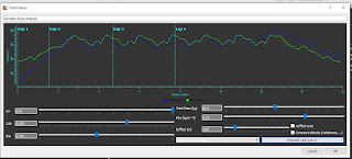
For this road testing, I imported the data into Golden Cheetah to perform the VE analysis.  I concluded that my CdA was 0.393 m^2 and my rolling resistance coefficient (CRR) on tarmac at 45 psi was 0.0100.

Off-road VE testing and venue

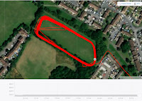
I then rode about a mile to the south, to a grassy field near my house, to perform the off-road testing.

It's worth noting that I did this testing during April 2020, which was at the start of the COVID-19 pandemic.  At the time, there were a lot of government-imposed restrictions in place, including a requirement for everyone to stay at home except for one exercise session per day.  As a result the field was fairly quiet, with just the occasional dog walker.  This allowed me to maintain a consistent line around the field and I didn't have any interruptions. 

Testing Protocol

My testing protocol is described in full below.  This can also be found in a post and subsequent discussion on the Slowtwitch Platypus Thread, on Page 20, which is a forum page dedicated to discussing the Virtual Elevation testing amongst cycling enthusiasts.  

- Stages 2nd generation left hand crank-based power meter. This is not ideal, to use a single-sided power meter, but it's all I've got.
- Tyre pressures measured with a digital Topeak pressure gauge. Possibly not accurate, but hopefully consistent.
- Garmin speed sensor. I used a constant value for the circumference in my Garmin head unit throughout the test, but then post-processed the results later to adjust the speeds based on the different measurements of when diameter for the different tyre pressures.
- Air density: Pressure from the weather forecast app. Temperature from the Garmin head unit.
- 0.97 transmission efficiency assumed throughout.
- Bike + rider weighing before and after the ride.
- No adjustment for wind. Sessions 1-3 in the chart were done with the forecast wind being 10-15mph. From what I've read, the ground level wind speed is less than the forecast wind speed by about half. My hope is that it would be consistent enough to give good enough increments between the pressures, even if the absolute numbers might be affected by the wind.

Tarmac runs
1) Tyres inflated to 45 psi.
2) 6 x laps of a tarmac oval loop, each lap 1 mile in length. First 3 laps done at ~230W, next 3 laps done at ~130W. No traffic.
3) VE analysis done in Golden Cheetah and Excel to check they give the same result, to check I haven't made a mistake in my Excel equations.
4) CdA and CRR determined post-ride so there is no elevation loss or gain over the six laps, trying also to keep the same flatness for the sets of fast and slow laps. The CdA derived from this analysis, 0.393, was then used for the VE analysis for the grass runs.

Grass runs
Straight from the tarmac runs, I cycled about 1 mile to a local grass field, roughly the size of a football pitch.
1) I checked the pressure before starting at 45 psi.
2) Accelerated up to speed before the maximum elevation point of the lap. Pressed the start/stop on the Garmin about 5-10 seconds before the max elevation point.
3) 3 laps at ~230W, followed by 3 laps at ~130W. I changed gear only once at the transition between fast and slow sets of laps, to keep the cadence reasonable. The time to do six laps was 7-8 minutes. I tried to follow a consistent line, but I had to avoid an occasional dog walker, approximately once every 5 laps (and these days trying to give people at least 5 metres of space!)
4) After the max elevation point at the end of the 6th lap, I continued for ~10 seconds, and pressed start stop on the Garmin.
5) Stopped in the shade. I avoided direct sunlight when stopped to prevent the sun warming the tyres. I checked the pressures, before then reducing the pressure by 5psi ready for the next run. I could get it within 0.5psi of the target. If I overshot the reduction for the first tyre (e.g. 39.5psi), I compensated by leaving the other tyre half a psi higher (e.g. 40.5psi). I chose to reduce pressure, rather than increase it, because I was concerned that pumping the tyre up might increase the internal air temperature and possibly the tyre wall temperature. Letting pressure out was also easier.
6) Step 2 onwards was repeated for 45 psi down to 15 psi in steps of 5 psi.
7) I then went home (<1 mile away), pumped the tyres back to 40 psi with a track pump, returned and followed the same protocol, but in 10 psi steps (40, 30, 20 psi). I wanted to do these repeats because I hadn't done an ABAB type test, and also because the grass was becoming increasingly flattened, which I think might have affected the CRR.
8) I also did a few repeats two days later, on a less windy day (~5mph wind according to the forecast)
9) CRR values were obtained to give no elevation gain/loss over the 6 laps, using the fixed CdA of 0.393. I obviously tried to keep the same kit and position on the bike throughout.

Results and discussion

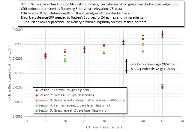
The results shown above surprised me somewhat.  The grass and the underlying surface felt reasonably smooth as far as off-road riding is concerned, with few bumps.  I was therefore expecting the suspension losses to be small.   What surprised me therefore is that there is no minimum in the plot, no optimal pressure.  It's clear that the lower the pressures, the lower the rolling resistance.  It seems the conventional wisdom of cyclocross racers, to go as low as possible with tyre pressures, may be right for rolling resistance as well as for traction.

I had a short discussion about these results with some of the experts on the SlowTwitch forum.  Tom Anhalt made an interesting comment that studies done for the Swiss MTB team a few years ago concluded the same way, that lower pressure is best.  He also said that the deformation of the surface (the ground, grass and dirt in this case) may be a large contributing factor, which in contrast is a negligible effect for the road.  This was a really interesting insight, and made me realise that for off-road riding, in addition to tyre hysteretic losses and suspension losses, there is a third source of rolling resistance, and that's hysteretic losses in the ground.  For anybody that has even tried cycling on sand, you'll be very aware that these hysteretic losses in the ground can be rather large!

Conclusion

The results showed me that I need to run my tyre pressures as low as possible.  The limit, to how low I could go, is however governed by a couple of factors:

• Tyre Stability: I found that below 20psi the tyre rolled around badly on the rim when cornering.  In these situations, a tubeless tyre can also 'burp' air, which can end a race if it happens a few times.
• Pinch flats: Even running tubeless, running very low pressures means that hitting rocks and hard obstacles can cause pinch flats in the tyre casing that won't seal.

As a consequence of seeing these results though, I am now running my tyre pressures much lower than before, and flirting with that limit for pinch flats and tyre stability.  To try to avoid those problems, and to facilitate lower pressures, I'll be trying out foam tyre inserts in the future.

Time trial saddle bag modification

Modified Saddle Bag for Time Trials

This is my low-drag saddle bag modification that I use on my time trial bike.

I need to have a saddle bag for my local evening 10-mile time trials, which start 5-10 miles away from my house, to carry a spare tube and some basic tools.  I don't have pockets in my skinsuit unfortunately.

The standard Topeak ProPack saddle bag, shown in the photo below, sits below the saddle, in the wind.  It always irked me that the nicely aero-profiled seatpost on my TT bike was spoiled by a large lump of a saddle bag sitting directly behind it.

Original Unmodified Topeak Saddle Bag

Now, with the extension I made for the saddle bag, using some timber offcuts, it should be lower drag.  It doesn't change the drag coefficient of the saddle bag, of course, but it now sits in the wake of my backside, so the dynamic pressure and the resulting drag (in Newtons) should now be lower than in its original position. 

I later modified it further, to have a red light on the back too, to comply with CTT regulations requiring a rear light.

Bike upgrades - Which offer the best value for money?

I did this analysis in 2016.  In fact, it was the first significant piece of bicycle performance analysis that I did, or at least, it’s the first study that's worth writing about.  The objective was to calculate which road bike upgrades offered the best value for money, in terms of making me faster on the bike.

I have been a keen cyclist for years, since about 1994 when I bought my first bike, a cheap £200 mountain bike.  In those first 15-20 years of recreational cycling, I frequently upgraded my bike(s) with new and better components. Like many other people during that era, I focussed on making my bikes lighter.  I was a bit of a weight weenie in those days, I'm ashamed to say.  Sadly, I can’t even say that my fitness justified the attention to detail that I put into my bike upgrades.

In the winter of 2015/2016, I realized that I knew everything necessary to model the forces and power losses that occur when riding a bike, and I was therefore able to analyse and quantify how much benefit could be achieved by making various improvements to either the bike, the kit or it's rider.  Doing so would mean that I had the possibility to check how beneficial all those weight savings had been on my cycling performance and how beneficial other types of improvement would be.  In turns out that I was in for a bit of a shock...

Method

My previous blog post explains the Excel-based method I created to model the power required to propel a bicycle at a certain speed and for certain set of conditions. That performance model development was a precursor to the analysis described in this post.  The Excel-based performance model also allows the power delivery/speed profile to be optimised for a prescribed cycle route (i.e. a gradient profile).  This optimisation functionality is important, because changes in bike equipment might lead to a slightly different optimised power profile that achieves the fastest bike speed (or in terms of how the actual computation is done, a slightly different optimised speed profile that achieves the prescribed average/normalised power constraint).

Re-optimisation example

The example below illustrates this, for a case where 2 kg is removed from the bike weight.

Case 1 in the table below is the optimised power profile for a 80km route described in the previous blog post, with the speed profile optimised to maximise the average speed (i.e. minimise ride time) for a prescribed normalised power of 200W.  In case 2, the weight is reduced by 2 kg, but the same speed profile is maintained. This results in a reduced normalised power of 197.294W, so a saving of about 3W (i.e. 2kg weight saving gives a 3W saving at the same speed).  For case 3, the same 197.294W normalised power is used as a constraint, and the speed/power profile is re-optimised.  This gives a small 3.6 second time improvement.

Although this re-optimisation change is very small, I wanted to do the power profile re-optimisation for each bike modification analysed to provide the best like-for-like comparison.  I also couldn't be sure that some bike modifications wouldn't affect more significantly the optimised power/speed profile.  I also think it's more relevant to know the speed improvement associated with a modification, for a fixed power, rather than a power improvement, since we tend to ride at a given power target/limit (our maximum capability) instead of targeting speed. The speed improvement is only achieved in my Excel model by re-running the optimisation.

                                     Bike weight        Avg Power       Normalised Power       Time           NP improvement

1) Optimised Power                 7 kg                192.6 W                 200.0 W         2 hrs 51.11 mins                -

2) Same speed profile as 1     5 kg                191.7 W                 197.3 W         2 hrs 51.11 mins             -2.7 W

3) Optimised speed profile     5 kg                191.7 W                 197.3 W         2 hrs 51.05 mins             -2.7 W

Bike modifications analysed

For the modifications I analysed, I considered a range of changes to the bike that would affect one of the forces of resistance acting on a bicycle:

• Aerodynamic resistance - Expressed via the CdA value (drag coefficient multiplied by frontal area) in the model. Items like aerodynamic helmets, deep section wheels, skinsuits etc.
• Rolling resistance - Expressed via the CRR (rolling resistance coefficient) value. Items like cheap versus expensive tyres, mountain bike tyres versus road tyres, inner tubes etc.
• Weight effects - Generally only affect the bike performance when riding uphill, but there is also a very small effect on rolling resistance on the flat too. 

In addition, I also looked at power changes, which would come from fitness improvements.  Again, the objective of all this was to understand relative differences between these changes.

Data sources

At this point, it's worth mentioning where I got my data from:

• For aerodynamic changes, I reverse-engineered the 40km time savings quoted by Specialized in their Wind Tunnel YouTube series.  I did this by iteratively determining the CdA reductions in my model needed to achieve the 40km time savings that the guys at Specialized quote.
• For rolling resistance changes, I took data from bicyclerollingresistance.com.
• For weight changes, although most changes were arbitrary changes like 1kg or 5kg reductions, I equated this to tangible changes like the cost of buying a more expensive groupset by looking at price data on Wiggle and weight data from bike component manufacturers such as Shimano.  For example, a Ultegra grouset will cost around £400-500 more than a 105 groupset, but will save around 200-300g.

Routes considered for analysis

I considered the same three fictional routes that I described in my previous post. Most of the items were analysed for Route 1, which is typical of many medium length sportives that might be done in the UK.  Results for routes 2 and 3 give some indication how sensitive the results are to the amount of climbing, which can be interesting because, for example, the effects of weight reductions on flat routes are almost negligible.

Route 1: Typical short/medium sportive - 80km route, 1000m of climbing, 200W normalised power.

Route 2: 40km TT - 40km perfectly flat route, 250W normalised power.

Route 3: Hilly route: 40km route with 900m of climbing, 250W normalised power

Baselines values

The various modifications analysed were considered relative to the following set of reference conditions:

• Air pressure = 1012.5 mbar (i.e. International Atmosphere sea level pressure)
• Air temperature = 20 degrees C
• Air density = 1.203 kg/m3 (calculated from the above pressure and temperature)
• Bike weight = 7kg
• Rider Weight = 11st 7lbs (161 lbs or 73.2kg)
• CRR = 0.045
• CdA = 0.36 m^2

Results

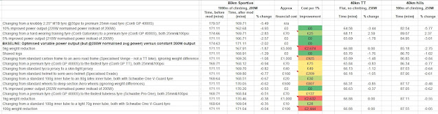
The table below shows the results for a number of bike modifications, with percentage time improvements ("% change" column) calculated either relative to the baseline setup above, or versus a degraded setup.

The cost effectiveness column called "cost per 1%" shows which modifications offer the best ride time improvement (or average speed improvement) for the money.  Green and yellow boxes show the best value for money modifications, whereas red items are poor value for money.

Improvements and cost effectiveness of various bike modifications

 There are a few key takeaways from this study:

• Power improvements: If you can improve your power, through improved training etc, at no extra cost then that is a very effective way to improve your average speed. For the 80km route, a 5% power improvement gives a 2.57% speed improvement.

• Optimised power: As discussed in my previous blog post, even if you are not any fitter, applying more or less power at the right time (i.e. optimising your power delivery) gives a significant 2.02% average speed improvement versus a constant power approach, even though the normalised power is no different.

• Rolling resistance improvements: By far, the best value for money upgrade you can make to a bike is improvements to your tyres and tubes.  Upgrading tyres and tubes will typically provide a cost effectiveness in the region of £30 per 1% improvement.  Even if you start from good tyres, like Conti GP 4000s tyres, upgrading to the best tyres is still less than £100 per 1% improvement.

• Weight: On the other hand, buying expensive components that will make your bike lighter are extremely poor value for money.  I have used the assumption of £1 per gram saved, which is a typical price you'll pay when going for a next tier groupset for example such as buying Dura Ace instead of Ultegra.  Spending £1000 to save 1kg will improve you average speed by only 0.38%, so that's around £2000-£3000 per 1% improvement!

• Aerodynamic improvements: The value for money of aero improvements is in the middle, with aero wheels and aero frames being quite costly, per 1% improvement, but aero helmets being a more cost effect upgrade.  Getting a tighter fitting jersey is a very cost effective improvement, rivalling the tyre and tube upgrades in terms of bang for your buck.

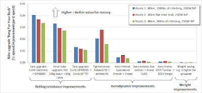
The numbers in the table above are a little difficult to read, admittedly, so I pulled a few of them into the chart to show visually how certain improvements are significantly better than others, in terms of value for money:

From this chart, it's clear that buying upgrades to improve rolling resistance is money well spent.  The aero improvements shown all give broadly similar average speed improvements in absolute terms, as said in the Specialized video with their time-saving-over-40km metric.  However, buying a tighter fitting jersey will be about one tenth the price of aero wheels or a new bike frame, so clearly a tight fitting jersey represents much better value for money.

As for weight improvements?  Well, since the bars on the right hand side of the bar chart are barely visible, spending money to make your bike lighter is extremely poor value for money, when it comes to actually going faster.  It seems that all the money I spent on lightweight components for many years was, sadly, a unwise choice.

Trades

It's finally worth showing some 'trades', i.e. what changes are equivalent, in terms of the resulting bike speed improvement.  These values have been obtained from the results above and their associated changes to either power, weight, drag or rolling resistance.

A 1% speed increase is achieved by:

Either a...   1.95% power increase

     Or a...    0.00077 CRR reduction

     Or a...    0.0153 m^2 CdA reduction (=4.3% CdA reduction)

     Or a...    2.67 kg weight reduction

 

Conclusion

In summary, spend your money on fast tyres and tubes as a priority, then upgrade to a tight fitting jersey.  For around £150, buying fast tyres, latex tubes and a tight jersey could improve your speed by 4-5%, depending on your starting point.  On the other hand £150 spent on lightweight components won't even improve your speed by 0.1%!

Finally, improving your power output, either by getting fitter to raise your power, or by optimising your power delivery, is a very effective way of going faster on the bike.

What’s the fastest way to ride a cycling route?

This was was the first piece of cycling performance analysis that I did, back in 2016.  A few months before that, in late 2015, I had bought a power meter for my road bike.  I really liked the data that it provided, allowing me to pace my rides with more precision.  I quickly began to question, though, how should I pace a ride to achieve the fastest time, i.e. the highest average speed?  Should I try to keep my power constant, regardless of the terrain and wind conditions, or would it be quicker to increase the power on some sections of the route?  We often hear that for time trials the fastest time is achieved by holding the highest possible fixed power, instead of going 'too hard' at the start.  However, most time trials are held on flat routes, and I had a feeling that the constant power approach may not be best for hilly routes.

This is question is essentially an optimisation problem: What is the optimal way to deliver the power to minimise ride time (i.e. maximise average speed) for a set of constraints.  I decided to see whether Microsoft Excel's built-in optimiser could solve this kind of optimisation problem.

I should point out that, at this time, I wasn't aware of BestBikeSplit.com.  A couple of years after I did this work I heard about BestBikeSplit on the TrainerRoad podcast and discovered that it does something very similar to my Excel spreadsheet, albeit in a slicker commercial package.  In fact, I'm not sure which year BestBikeSplit was originally developed, but I wasn't aware of it when I developed this Excel-based bike power optimiser.  A future blog post will show comparisons between my my Excel optimiser and BestBikeSplit, showing that they both give similar optimisation results.

Bicycle Power Modelling

The starting point of my Excel based power optimiser was to build a model that calculates the required power to propel a bike.  The equations of motion that describe the forces on a bike, and hence the power required to move it, are shown below.

This is another situation where I derived something myself, the equations below, and then some years later discovered that this model of the forces acting on a bicycle had been derived previously (not surprisingly). See here for Jim Martin's paper.

Power = (Fa + Fg + Fr + Fi)*V

   Where:

   Fa = Aerodynamic drag force (N)
   Fg = Gravitational component force (N)
   Fr = Rolling resistance force (N)
   Fi = Inertia force (N)
   V = Velocity (m/s)

   and:

   CdA = Drag area of the bike+rider (m^2)

   Cr = Coefficient of rolling resistance
   rho = Air density (kg/m^3)
   m = Mass of bike+rider (kg)
   t = time (s)
  g = Acceleration due to gravity (=9.81m/s^2)  

This power model was validated by comparing the power predicted by this model against the measured powers that I recorded during three Strava segments; 2 flat segments and an uphill segment:

1) Weston Hill, near Bath, South West England:

https://www.strava.com/segments/6665281 : 1.578 km, 10.3% gradient.

Real life: 18/07/15, 7 mins 35 secs (8.0 mph),  20 degC,  80.6 kg, 313 W average power

Model:  8.0 mph gives a power requirement of 314W using CdA=0.36m^2, Cr=0.0045

-> +1W (+0.3%) discrepancy

2) U102 out and back time trial segments, near Bristol: 

https://www.strava.com/segments/1286195?filter=overall : 5.60 km, -0.1% gradient.

Real life: 18/08/15, 8 mins 32 secs (24.5mph),  17 degC,  80 kg, 2 mph estimated tailwind, 267 W average power

Model:  24.5 mph (with 2 mph tailwind) gives a power requirement of 273 W using CdA=0.36m^2, Cr=0.0045

-> +6W (+2.2%) discrepancy

https://www.strava.com/segments/4769147?filter=overall : 7.42 km, 0.0% gradient.

Real life: 18/08/15, 13 mins 1 secs (21.3mph),  17 degC,  80 kg, 2 mph estimated headwind, 267 W average power

Model:  21.3 mph (with 2mph headwind) gives a power requirement of 260W using CdA=0.36m^2, Cr=0.0045

-> -7W (-2.7 %) discrepancy

The agreement between the model and measured (real life) powers agree within a few percent.  For the hilly segment, the model predicts the power requirement very well (a 1W or 0.3% discrepancy).  For the two flat segments, the model overpredicts the power requirement for the 'out' leg of the TT course and and underpredicts it for the return leg, due to the estimated wind effects.  If I were to tweak the headwind by just 0.3 mph (bearing in mind that I had to guess the headwind speed of 2 mph) then the model is spot on, within a few tenths of a percent for both out and return legs. Therefore, it can be concluded that overall the model and the values selected for CdA and Crr (drag area and coefficient of rolling resistance, 0.36m^2 and 0.0045 respectively) accurately simulate real life riding.

This model validation step was an important precursor to any subsequent use of the model for further investigations, as described in the next section.

Optimal power delivery

My Excel-based power model simulates a bike ride by splitting it up into several 'segments'. For each segment, which has a specified distance and gradient, the speed is set either by the user or by the Excel optimiser.  Then, the model calculates the power for each segment for the chosen speeds, assuming steady-state conditions.  Essentially, this neglects speed and acceleration transients between segments, which I understand is the same assumption made also by BestBikeSplit.

The powers for all of the segments can be time-averaged to calculate the overall average power for the ride, and this is the result that the optimiser is trying to minimise (or to look at it another way, it tries to maximise the average speed for a fixed average power).

I also included an approximate estimate for normalised power, since it's often that case that normalised power is the metric that we want to minimise or control instead of average power, to reflect the physiological cost of the ride.  My spreadsheet calculates only approximate normalised power though, because instead of using the 30-second average power to derive normalised power, it effectively uses 1-second power.  This is not too much of an issue, though, because most segments I used for these studies were much longer than 30 seconds, so there were no short segments where the time would be less that 30 seconds, where the normalised power calculation would have been significantly impacted.  Therefore, the approximate calculation of normalised power is fit for purpose.

The optimiser can be used to either target an average power number or a normalised power number, whichever is preferred.  In the subsequent example I chose to target a given normalised power.

Routes for optimiser

I created three fictional routes, to see how the optimised power would differ for different types of rides:

Route 1: Typical short/medium sportive - 80km route, 1000m of climbing, 200W normalised power.

Route 2: 40km TT - 40km perfectly flat route, 250W normalised power.

Route 3: Hilly route: 40km route with 900m of climbing, 250W normalised power

The profile for Route 1 (80km, 1000m of climbing) is shown below:

The profile for Route 3 (40km, 900m of climbing) is shown below:

Results: Constant power versus optimised power

For Route 1 (80km, 1000m climbing), the optimised power profile, targeting 200W normalised power is shown below (upper chart), compared with the fixed power profile (lower chart).  It is clear the that optimiser has determined that it is optimal to increase the power when ascending hills and reduce the power when descending hills.

                                 Average Power        Normalised Power             Time                  Improvement

Constant Power                  200.0 W                     200.0 W                 2 hrs 54.6 mins                  -

Optimised Power                192.6 W                     200.0 W                 2 hrs 51.1 mins                2.0%

An optimised power delivery achieves a 2.0% improvement (three and a half minutes) for the same normalised power of 200W.  Note that the same normalised power means the optimised power delivery has a 7.4W lower average power, at 192.6W.  Since it has the same normalised power and a lower average power, the optimised power profile would I think not only be faster, but would feel similar or easier than the constant power profile.

For Route 2 (40km, perfectly flat route), the optimised power profile, targeting 250W normalised power is exactly the same as the constant power profile, i.e. it is optimal to ride at at a fixed power of 250W.  This is not surprising, because the optimum power profile is a result of changes to the riding conditions. No changes in terrain or wind mean the optimum is a constant power profile.  If the terrain or wind were to change along the route, the optimal power at any particular point in a ride would change also, as can be seen for Route 1 above and Route 3 below.

For Route 3 (Hilly route: 40km route with 900m of climbing), the optimised power profile, targeting 250W normalised power is shown below (upper chart), compared with the fixed power profile (lower chart).  As for Route 1, the optimiser has again determined that it is optimal to increase the power when ascending hills and reduce the power when descending hills.

                                 Average Power        Normalised Power              Time                  Improvement

Constant Power                  250.0 W                     250.0 W                 1 hr 30.0 mins                  -

Optimised Power                237.5 W                     250.0 W                 1 hr 27.6 mins                2.7%

'Too hard' power                 224.7 W                     250.0 W                 1 hr 28.0 mins                2.2%

As for Route 1, the optimised power delivery achieves a significant improvement for the same normalised power.  In this case, the improvement is slightly more than for Route 1, at 2.7%.  Again, this improvement is achieved by pushing slightly harder on the climbs and then backing off slightly on the descents.

What happens, though, if you push even harder on the hills (labelled the "Too hard" case above)?  I took the optimised power profile shown in the plot above and increased the amplitude of the speed variation (fixed power versus optimised power) by 50%, then made a 0.2 mph global adjustment to the speed to keep the normalised power at exactly 250W.  For example, for the steep 10% gradient climb in the middle of the route, the climb is done at 6.64 mph for the constant 250W power profile,  7.48 mph at the optimum power of 283W, and 7.72 mph at the 'too hard' power of 293W.

The overall result is a ride time that's still better than the constant power approach, but is worse than for the optimum power profile. This also is a useful quick-and-dirty check that the optimiser is working as intended.  The very subtle differences in the chosen powers for the 'optimum' and 'too hard' power profiles (283W vs 293W) shows that it's difficult to select the optimum power based on guesswork alone, and it's easy to go too hard on hills. Anecdotally, this is something I see a lot of recreational riders doing on sportives, riding overly hard on the climbs.

Conclusion

My Excel-based power optimiser uses fairly simple modelling of the forces acting on a bike to estimate the required power for a given speed. This model has been validated based on real-life rides and measured power data.

The optimiser can determine the optimum (best) use of a person's power for any cycle route. The results show that improvement in time and average speed can be made by pushing harder (above average or normalised power) on the climbs and easing off on the descents (below avg or normalised power). This tends to be what riders do naturally when riding, but the optimisatiosn studies have also shown that it's difficult to judge how much harder and easier those power variations should be to achieve the best (optimum) ride.

The optimum power profile provides a significant performance improvement compared with a constant power approach.  2-3% improvements are possible, which may not sound like large improvements, but a 2-3% improvement is equivalent to about 5% power improvement, or a huge 5-6kg weight saving*.

* A future blog post will show these effects and the best way to spend your money on bike improvements.  In fact, this power optimisation model was a precursor for doing those best-bang-for-your-buck studies.

Finally:  Observant people will notice that that my power modelling doesn't have a correction for transmission losses, so it implicitly models a perfectly efficient transmission, or the power required at the rear hub, not power at the pedals. This was an oversight on my part. However, although it will affect the absolute predicted powers/speeds and therefore the CdA and CRR tuning, I don't believe it will affect the overall conclusions of this study.