Upgrade recommendations for a friend

In a 2016 blog post, I described an analysis that concluded about the best value for money upgrades that people can buy for their road bikes.

Last week, in my previous post, I described the power delivery optimisation that I did for my friend Steve, to show how much faster he could go just by changing when he pushed harder on his favourite bike route and when to ease off.  I followed this up with a quick study to show how much benefit could be achieved with certain bike and kit upgrades.

The analysis I did was basically the same as the 2016 analysis, except it was done for Steve's lunchtime bike route, instead or three generic bike ride profiles.  The results are shown in the bubble plot above.  I've shown it with upgrade price on the x-axis, and the equivalent power saving in the y-axis.  Items that represent the best value for money (Watt saving per £ spent) have the largest bubbles.

The conclusions are similar to those in the 2016 blog post.  Buying latex tubes represents excellent value for money, probably the best there is.  On the other hand, paying extra money for a lighter groupset (if it has no additional functional benefits) is a really bad way to spend your money, if improved cycling performance is your priority.

Power delivery optimisation for a real-life cycling route

In a previous blog post (here) I described a power delivery optimisation analysis that I did back in 2016.  In that work I showed that, using a simple Excel-based optimiser, it's possible to make significant performance gains, a 2-3% improvement in that case, simply by optimising the power delivered during a bike ride for the same normalised power.  In other words, making the most of what you've got.  These improvements were the versus the 'baseline' situation where the ride was done at a fixed (not varying) power output with the same normalised power.  A 2-3% improvement may not sound like much, but to put this into context, that performance gain is equivalent to a 5% power improvement, for a fixed power delivery.  Alternatively, it's equivalent to a 5-6kg of weight loss, which is significant.

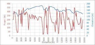
That study was done for a fictional 80km route having 1000m of elevation gain.  In 2020, a friend of mine, Steve, who's also an engineer, asked me if there was a better way for him to ride his favourite lunchtime cycle loop.  To give him some advice, I decided to try putting his bike route into my Excel optimiser to see what it would give.  By optimising his power, using the optimised power profile shown in the plot above, he could make an impressive 3.8% time saving and speed improvement, compared with riding the route at a fixed (constant) power.  This blog post describes that work in more detail.

Route setup

First I extracted my friend Steve's lunchtime route from Strava, as a GPX file.  That Strava output gave 276 waypoints on the route, with longitude, latitude and elevation data.

For my optimiser to work, I needed to reduce the number of points to 137 points, which is a number of segments that would be compatible with what Excel's optimiser can handle.

Steve's best time for this ride was 29 minutes, 42 seconds, which was an average speed of 31.8 kph.  I obtained a few other parameters from the  Strava file for his personal best time, then I needed to guess a few others:

Ambient temperature = 6 deg C  (from Strava)
Ambient Pressure = 101.25 Pa  (assumed)
Bike + Rider = 97.5 kg  (estimated)
Mechanical efficiency = 97.5%  (assumed)
No wind  (assumed)

Comparison with BestBikeSplit

As a first check that my optimiser was doing something sensible, I compared the output with BestBikeSplit.  BestBikeSplit does something very similar, so both methods should give reasonably similar results.  

BestBikeSplit assumed a rolling resistance coefficent (CRR) of 0.00622 and a CdA of 0.3424 [an explanation of CdA can be found here].  I used those two values in my own optimiser.  As can be seen from the plot on the left, both methods gave reasonably similar results for a normalised power of 239W:

BestBikeSplit: 29.8 kph average speed

My optimiser: 30.7 kph average speed

Qualitatively, the power distributions in those plots look similar.  The BestBikeSplit optimiser can split the route into only 50 segments, whereas my optimiser used 137 segments. This might be a reason why the average speeds differ slightly.  In any case, I was satisfied that this agreement was close enough.

Tuning CdA

I then tuned the value of CdA so that the optimised ride time was equal to Steve's best ride time.  Reducing CdA to 0.29 was enough to do this, to increase the average speed from 30.7 kph (for a CdA of 0.3424) to 31.8 kph for a CdA of 0.29.  A CdA value of 0.29 is a bit low for a recreational cyclist, in my experience, but Steve often rides with one of two colleagues, so 0.29 seems a reasonable value for his effective CdA, considering that some of the time he'd be riding in the draft of other people.

For this CdA of 0.29, and for a normalised power of 259.8W, I computed the "weighted average power" to be 241.0W and the average power to be 227.3W.

At this point I should note that the way in which Strava calculates weighted average power is not documented anywhere by Strava.  Weighted average values are generally higher than the average power values in my experience, but are always less than normalised power values.  Whereas normalised power is calculated by raising the power values to the power of 4, I assumed that weighted power is calculated by raising the power values to the power of 2.

So to summarise, I now had an optimised power profile (see plot on the left) that produced an average speed that is identical to Steve's PB effort (31.8kph) using the same weighted average power as he produced in real life (241W).  Of course, it's highly unlikely that he would have ridden the route at the optimum power profile, but for the purposes of this study, to quantify the benefits of optimising power, I think that's good enough.  As an observation, it's interesting to see that the power needed to produce this optimised performance varies significantly, from about 20W on the steepest downhill part of the route (-10% gradient) to about 370W on the steepest uphill part of the route (+8% gradient).  Incidentally, the average power and normalised power for this power delivery is 227W and 260W respectively.

The improvement that the optimised power delivery achieves, versus the baseline case of a fixed, non-varying, power delivery can then be calculated by re-running my optimiser with an additional constraint.

How much faster is the optimised power delivery?

I re-ran the optimiser with weighted average power set to 241W, as before, but this time I also set an additional constraint that the average power had to be 241W too.  This additional average power constraint effectively prevented any significant variation in the power, meaning that the power delivery effectively became almost constant at 241W, as shown in the plot above.

The speed of this ride, if performed at this fixed power of 241W, would be 30.6 kph.  This is 1.2 kph slower (3.8% slower) than for the ride done at the optimised power delivery.

Comparison to other improvements

The significance of this 3.8% improvement is not so obvious, but can be put into context by calculating the effect of other improvements:

+10 Watts increase in weighted average power:            +0.7kph improvement (2.2% faster)

Butyl -> Latex inner tubes (-11% rolling resistance):      +0.3kph improvement (1.1% faster)

5 kg weight saving:                                                         +0.5kph improvement (1.5% faster)

Aero improvement through and aero helmet upgrade:   +0.2kph improvement (0.8% faster)

The speed improvements shown above make it clear how significant that 1.2kph (3.8%) improvement is from simply optimising the power delivery, applying the right amount of effort at the right time. 

Finally...

I was curious to see whether there is a relationship between optimum power and gradient.  Clearly, it's impractical, and will get kind of boring, to do this kind of analysis for every route that I might want to ride.  This work and previous work has shown that the optimiser determines that more power should be applied on the uphills, and less power on the downhills, but could there be a general rule? 

For the 137 segments of this route, I plotted on the left the optimum power versus the gradient.  It can be seen that the the points fall onto an smooth S-shaped trend line with no scatter.

Perhaps more useful is the plot below, which is the same data but plotted as the ratio of the optimum power to the average power.  

So for example, you can see that for an uphill section of the route with a gradient of 5%, you should be cycling at a power that's approximately 50% higher than your average power.  Then, for a downhill section, having 5% gradient, you should be at 25% of your average power.

Obviously, this optimum delivery assumes that the riding conditions (traffic, corners, etc) do not limit the speeds, and that is one important caveat on all of this.  Also there is no consideration of what is achievable by a rider.  For example, if the average power is close to a rider's threshold, then they would only be able to hold those optimal higher power on uphill parts of the course for short periods of time.  The optimiser is simply finding the best power delivery profile for the prescribed average power.  In principle, additional physiological constraints could be put into the optimiser, but I haven't tried doing that yet.

As a next step, I'd like to see whether this optimum power relationship holds true for other bike routes and for other cases where there changes are made to either the riding conditions, the bike or the rider.